MCMC Fit (using emcee)
This tutorial demonstrates how to perform a fit using the MCMC backend (emcee) and how to interpret the associated diagnostic plots.
Unlike classical optimizers such as lmfit or scipy.odr, the emcee sampler generates a distribution of parameter values rather than a single best-fit solution. This enables a deeper analysis of parameter uncertainties and correlations.
Note: The visualizations described in this section are only available when using the MCMC method.
1. Load the Data
Begin by opening the application and loading the dataset:
examples/data/two_gaussians_with_slope.csv
This file contains a signal composed of two Gaussians peak and a linear trend.
If desired, you can restrict the fitting range using the Xmin/Xmax tool in the toolbar.
2. Define the Model
In the Fit Formula dock, enter the following expression:
y = p0 * exp(-0.5 * ((x - p1) / p2)**2) + p3 * exp(-0.5 * ((x - p4) / p5)**2) + p6 * x + p7
This model combines two Gaussians functions with a slope and offset.
Tip: Run a Classical Fit First
Before switching to MCMC, it is strongly recommended to run a preliminary fit using a classical method (e.g. leastsq). This provides a good estimate of the initial parameter values.
MCMC sampling is sensitive to the starting point. Starting from uninitialized or poorly chosen values may cause:
- Slow convergence
- Divergence of walkers
- Inefficient exploration of the parameter space
By running a classical fit first, the initial guess (p0) used by emcee will be closer to the region of interest, leading to faster and more stable results.
You can then reopen the Fit Options, switch to emcee, and run the MCMC sampling using the values obtained from the initial fit.
3. Set the Fit Options
Click the Fit Options button to open the configuration dialog. Go to the Genral options tab.
- Select
emceeas the fitting method -
Recommended MCMC parameters:
-
nwalkers: 100 steps: 1000burn: 200thin: 5- Enable
is_weightedif your dataset includesY_err
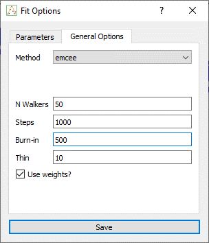
Click OK to confirm.
4. Run the Fit
Click the Fit button in the toolbar. Once the sampling is complete, the application will update the Results Dock and display the relevant plots.
5. MCMC Diagnostic Plots
Four types of plots are generated automatically:
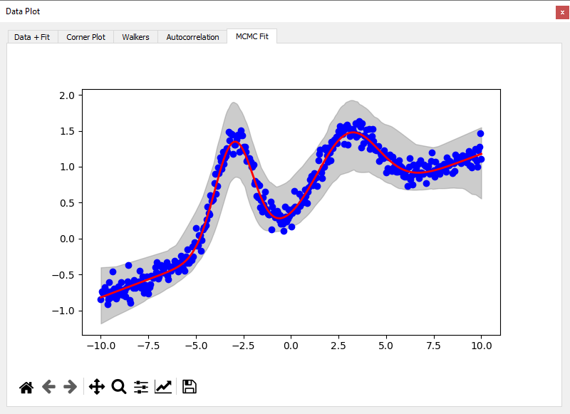
Confidence Band
- The median model curve is displayed.
- A shaded region represents the 99% confidence interval.
- This interval is computed using percentiles over 500 randomly selected samples.
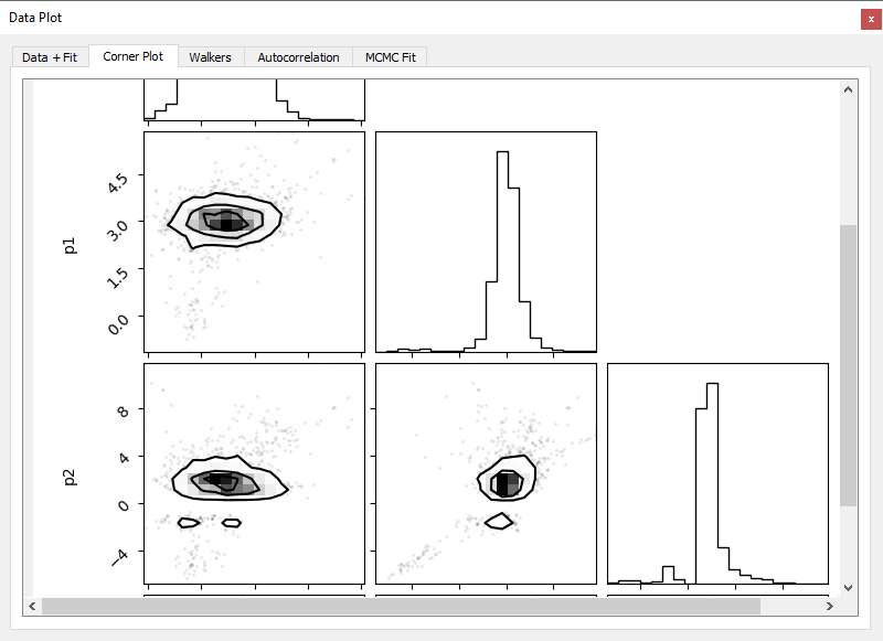
Corner Plot
- Shows marginal and joint posterior distributions for all parameters.
- Useful to evaluate uncertainty and parameter correlations.
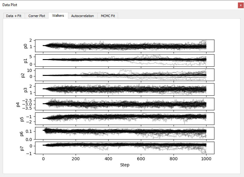
Walkers Plot
- Each walker trajectory is plotted per parameter.
- Helps assess convergence and sample mixing.
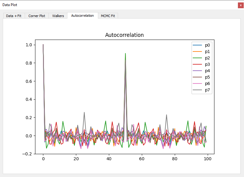
Autocorrelation
- Displays the autocorrelation as a function of lag for each parameter.
- Helps estimate the effective sample size.