Fitting a 2D Surface
This tutorial demonstrates how to use the 2D surface fitting mode to fit a model to data defined over a 2D grid. This is useful when your measurements depend simultaneously on two variables, and the response surface can be described by a global model of the form $z = f(x, y)$.
Step 1 – Load the data
Use File > Load Data and select:
examples/data/surface_fit_tuto.csv
This dataset includes:
X: the first independent variableY: the second independent variableZ: the observed value at each (X, Y) point
After loading, the application automatically switches to 2D mode, and the Fit Strategy selector appears in the control dock.
Select the strategy:
Fit surface (Z = f(X, Y))
Step 2 – Define the formula
We use a 2D Gaussian surface combined with an interaction term:
z = A * exp(-((x - B)**2 + (y - C)**2) / (2 * D**2)) + E * x * y
This model contains five parameters:
A: amplitude of the Gaussian peakB: center position along XC: center position along YD: width of the GaussianE: interaction term that introduces a cross-dependence between X and Y
This formula is global: it is fitted to all points simultaneously.
Step 3 – Run the fit
Click Fit in the fit control dock. The application will:
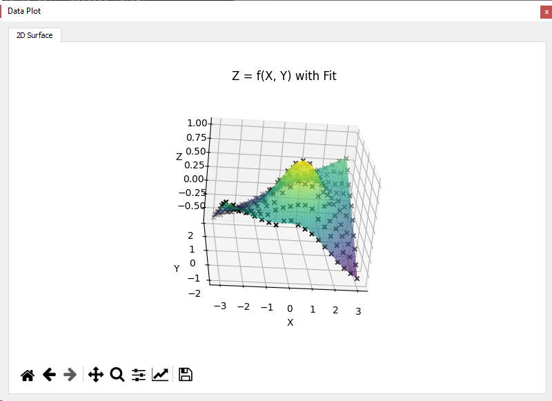
- Fit all data points using the selected method (default:
lmfit) - Display the raw data and fitted surface in a3D view with crosses for data and a surface for the fit
You can also switch to alternative methods:
odrfor orthogonal error regressionemceefor Bayesian sampling
For emcee, it’s often recommended to first run a classical fit to initialize the parameters.
Notes
This 2D surface fitting mode assumes that all variables x, y, and z are numeric and that the formula defines a continuous surface. Avoid sharp discontinuities or piecewise expressions when using this strategy.