Manual Fitting Mode
This tutorial introduces the manual mode, which allows you to visualize the effect of a formula and manually adjust its parameters using sliders — without launching an automatic fit. This mode is ideal for verifying formulas, exploring parameter behavior, and setting good initial guesses.
Step 1 – Load the data
Use File > Load Data and select:
examples/data/manual_fit_tuto.csv
This dataset includes:
X: the main sweep variableY: a secondary index (discrete)Z: the observed value for each (X, Y)
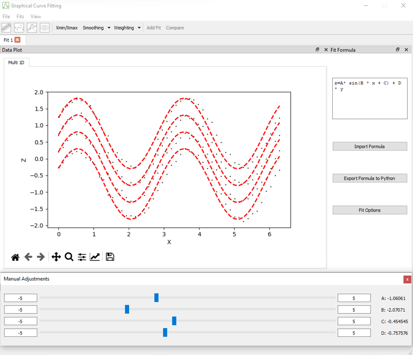
After loading, the application automatically enters Fit per Y and displays a set of curves indexed by Y.
There is no manual mode for 3d plots
Step 2 – Switch to manual mode
In the Fit Control dock, click:
Manual
This disables the "Fit" button and instead activates a slider interface for parameter adjustment. This allows real-time manipulation of parameters without optimization.
Step 3 – Define a formula
Try the following example:
z = A * sin(B * x + C) + D * y
Once entered, sliders appear for each parameter (A, B, C, D). You can now adjust them manually.
- Use the slider to change the value of the parameter
- The limits can be changed by clicking on the values at the ends of the sliders
Step 4 – Adjust the sliders
Each slider updates the plot in real time. You can:
- See how each parameter influences the curve
- Explore how well the formula matches the data visually
- Zoom/pan to inspect features in detail
If in 2D mode (i.e. Y is present), a curve is displayed for each value of Y.
Step 5 – Use it to set initial guesses
Once a visually good match is found:
- Switch to a fitting method such as
lmfit,odr, oremcee - The last slider values are retained as the initial guesses
- Click Fit to run the optimization from that point
This can significantly improve convergence and avoid local minima.
Why use manual mode?
- Quickly verify that the formula is well-formed
- Understand parameter roles and interactions
- Pre-tune parameters for faster and more accurate fitting
- Compare models before choosing one